Calcium Imaging 🎬

Introduction
In this tutorial, we will create fake data for a hypothetical optical physiology experiment with a freely moving animal. The types of data we will convert are:
Acquired two-photon images
Image segmentation (ROIs)
Fluorescence and dF/F response
It is recommended to first work through the Introduction to MatNWB tutorial, which demonstrates installing MatNWB and creating an NWB file with subject information, animal position, and trials, as well as writing and reading NWB files in MATLAB.
Please note: The dimensions of timeseries data in MatNWB should be defined in the opposite order of how it is defined in the nwb-schemas. In NWB, time is always stored in the first dimension of the data, whereas in MatNWB data should be specified with time along the last dimension. This is explained in more detail here: MatNWB <-> HDF5 Dimension Mapping.
Set up the NWB file
An NWB file represents a single session of an experiment. Each file must have a session_description, identifier, and session start time. Create a new NWBFile object with those and additional metadata. For all MatNWB functions, we use the Matlab method of entering keyword argument pairs, where arguments are entered as name followed by value.
nwb = NwbFile( ...
    'identifier', 'matnwb_ophys_tutorial', ...
    'session_description', 'mouse in open exploration',...
    'session_start_time', datetime(2018, 4, 25, 2, 30, 3, 'TimeZone', 'local'), ...
    'timestamps_reference_time', datetime(2018, 4, 25, 3, 0, 45, 'TimeZone', 'local'), ...
    'general_experimenter', 'LastName, FirstName', ... % optional
    'general_session_id', 'Mouse5_Day3', ... % optional
    'general_institution', 'University of My Institution', ... % optional
    'general_related_publications', {'DOI:10.1016/j.neuron.2016.12.011'}); % optional
nwb
nwb =
  NwbFile with properties:

                                             nwb_version: '2.9.0'
                                        file_create_date: []
                                              identifier: 'matnwb_ophys_tutorial'
                                     session_description: 'mouse in open exploration'
                                      session_start_time: {[2018-04-25T02:30:03.000000+02:00]}
                               timestamps_reference_time: {[2018-04-25T03:00:45.000000+02:00]}
                                             acquisition: [0x1 types.untyped.Set]
                                                analysis: [0x1 types.untyped.Set]
                                                 general: [0x1 types.untyped.Set]
                                 general_data_collection: ''
                                         general_devices: [0x1 types.untyped.Set]
                                  general_devices_models: [0x1 types.untyped.Set]
                          general_experiment_description: ''
                                    general_experimenter: 'LastName, FirstName'
                             general_extracellular_ephys: [0x1 types.untyped.Set]
                  general_extracellular_ephys_electrodes: []
                                     general_institution: 'University of My Institution'
                             general_intracellular_ephys: [0x1 types.untyped.Set]
     general_intracellular_ephys_experimental_conditions: []
                   general_intracellular_ephys_filtering: ''
    general_intracellular_ephys_intracellular_recordings: []
                 general_intracellular_ephys_repetitions: []
       general_intracellular_ephys_sequential_recordings: []
     general_intracellular_ephys_simultaneous_recordings: []
                 general_intracellular_ephys_sweep_table: []
                                        general_keywords: ''
                                             general_lab: ''
                                           general_notes: ''
                                    general_optogenetics: [0x1 types.untyped.Set]
                                  general_optophysiology: [0x1 types.untyped.Set]
                                    general_pharmacology: ''
                                        general_protocol: ''
                            general_related_publications: {'DOI:10.1016/j.neuron.2016.12.011'}
                                      general_session_id: 'Mouse5_Day3'
                                          general_slices: ''
                                   general_source_script: ''
                         general_source_script_file_name: ''
                                        general_stimulus: ''
                                         general_subject: []
                                         general_surgery: ''
                                           general_virus: ''
                                general_was_generated_by: ''
                                               intervals: [0x1 types.untyped.Set]
                                        intervals_epochs: []
                                 intervals_invalid_times: []
                                        intervals_trials: []
                                              processing: [0x1 types.untyped.Set]
                                                 scratch: [0x1 types.untyped.Set]
                                   stimulus_presentation: [0x1 types.untyped.Set]
                                      stimulus_templates: [0x1 types.untyped.Set]
                                                   units: []
Subject Information
It is recommended to store information about the experimental subject in the file. Create a Subject object to store metadata about the subject, then assign it to nwb.general_subject.
subject = types.core.Subject( ...
    'subject_id', '005', ...
    'age', 'P90D', ...
    'description', 'mouse 5', ...
    'species', 'Mus musculus', ...
    'sex', 'M' ...
);
nwb.general_subject = subject;
Optical Physiology
Optical physiology results are written in four steps:
Create imaging plane
Acquired two-photon images
Image segmentation
Fluorescence and dF/F responses
Imaging Plane
First, you must create an ImagingPlane object, which will hold information about the area and method used to collect the optical imaging data. This requires creation of a Device object for the microscope and an OpticalChannel object. Then you can create an ImagingPlane.
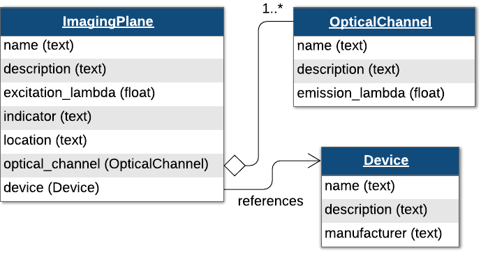
Create a Device representing a two-photon microscope. The fields description, manufacturer, model_number, model_name, and serial_number are optional, but recommended. Then create an OpticalChannel and add both of these to the ImagingPlane.
device = types.core.Device( ...
    'description', 'My two-photon microscope', ...
    'manufacturer', 'Loki Labs', ...
    'model_number', 'ABC-123', ...
    'model_name', 'Loki 1.0', ...
    'serial_number', '1234567890');

% Add device to nwb object
nwb.general_devices.set('Device', device);

optical_channel = types.core.OpticalChannel( ...
    'description', 'description', ...
    'emission_lambda', 500.);

imaging_plane_name = 'imaging_plane';
imaging_plane = types.core.ImagingPlane( ...
    'optical_channel', optical_channel, ...
    'description', 'a very interesting part of the brain', ...
    'device', types.untyped.SoftLink(device), ...
    'excitation_lambda', 600., ...
    'imaging_rate', 5., ...
    'indicator', 'GFP', ...
    'location', 'Primary visual area');

nwb.general_optophysiology.set(imaging_plane_name, imaging_plane);
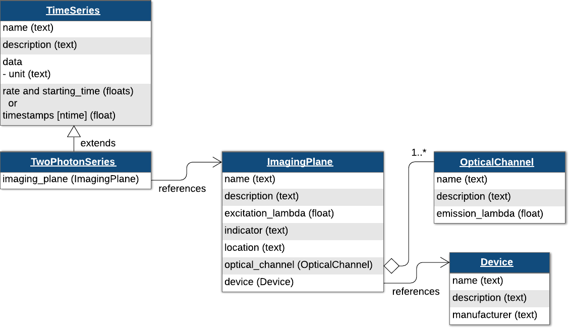
Storing Two-Photon Data
You can create a TwoPhotonSeries class representing two photon imaging data. TwoPhotonSeries, like SpatialSeries, inherits from TimeSeries and is similar in behavior to OnePhotonSeries.
InternalTwoPhoton = types.core.TwoPhotonSeries( ...
    'imaging_plane', types.untyped.SoftLink(imaging_plane), ...
    'starting_time', 0.0, ...
    'starting_time_rate', 3.0, ...
    'data', ones(200, 100, 1000), ...
    'data_unit', 'lumens');

nwb.acquisition.set('2pInternal', InternalTwoPhoton);
Storing One-Photon Data
Now that we have our ImagingPlane, we can create a OnePhotonSeries object to store raw one-photon imaging data.
% using internal data. this data will be stored inside the NWB file
InternalOnePhoton = types.core.OnePhotonSeries( ...
    'data', ones(100, 100, 1000), ...
    'imaging_plane', types.untyped.SoftLink(imaging_plane), ...
    'starting_time', 0., ...
    'starting_time_rate', 1.0, ...
    'data_unit', 'normalized amplitude' ...
);
nwb.acquisition.set('1pInternal', InternalOnePhoton);
Motion Correction (optional)
You can also store the result of motion correction using a MotionCorrection object, a container type that can hold one or more CorrectedImageStack objects.
% Create the corrected ImageSeries
corrected = types.core.ImageSeries( ...
    'description', 'A motion corrected image stack', ...
    'data', ones(100, 100, 1000), ...  % 3D data array
    'data_unit', 'n/a', ...
    'format', 'raw', ...
    'starting_time', 0.0, ...
    'starting_time_rate', 1.0 ...
);

% Create the xy_translation TimeSeries
xy_translation = types.core.TimeSeries( ...
    'description', 'x,y translation in pixels', ...
    'data', ones(2, 1000), ...  % 2D data array
    'data_unit', 'pixels', ...
    'starting_time', 0.0, ...
    'starting_time_rate', 1.0 ...
);

% Create the CorrectedImageStack
corrected_image_stack = types.core.CorrectedImageStack( ...
    'corrected', corrected, ...
    'original', types.untyped.SoftLink(InternalOnePhoton), ... % Ensure `InternalOnePhoton` exists
    'xy_translation', xy_translation ...
);

% Create the MotionCorrection object
motion_correction = types.core.MotionCorrection();
motion_correction.correctedimagestack.set('CorrectedImageStack', corrected_image_stack);
The motion corrected data is considered processed data and will be added to the processing field of the nwb object using a ProcessingModule called “ophys”. First, create the ProcessingModule object and then add the motion_correction object to it, naming it “MotionCorrection”.
ophys_module = types.core.ProcessingModule( ...
    'description', 'Contains optical physiology data');
ophys_module.nwbdatainterface.set('MotionCorrection', motion_correction);
Finally, add the “ophys” ProcessingModule to the nwb (Note that we can continue adding objects to the “ophys” ProcessingModule without needing to explicitly update the nwb):
nwb.processing.set('ophys', ophys_module);
Plane Segmentation
Image segmentation stores the detected regions of interest in the TwoPhotonSeries data. ImageSegmentation allows you to have more than one segmentation by creating more PlaneSegmentation objects.
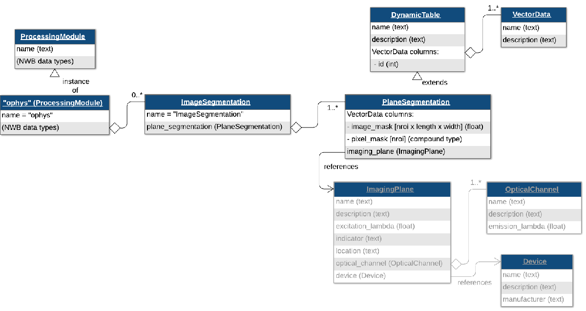
Regions of interest (ROIs)
ROIs can be added to a PlaneSegmentation either as an image_mask or as a pixel_mask. An image mask is an array that is the same size as a single frame of the TwoPhotonSeries, and indicates where a single region of interest is. This image mask may be boolean or continuous between 0 and 1. A pixel_mask, on the other hand, is a list of indices (i.e coordinates) and weights for the ROI. The pixel_mask is represented as a compound data type using a ragged array and below is an example demonstrating how to create either an image_mask or a pixel_mask. Changing the dropdown selection will update the PlaneSegmentation object accordingly.
selection = "Create Image Mask"; % "Create Image Mask" or "Create Pixel Mask"

% generate fake image_mask data
imaging_shape = [100, 100];
x = imaging_shape(1);
y = imaging_shape(2);

n_rois = 20;
image_mask = zeros(y, x, n_rois);
center = generateCenterCoords(90,2,n_rois);
for i = 1:n_rois
    image_mask(center(1,i):center(1,i)+10, center(2,i):center(2,i)+10, i) = 1;
end

if selection == "Create Pixel Mask"
    ind = find(image_mask);
    [y_ind, x_ind, roi_ind] = ind2sub(size(image_mask), ind);

    pixel_mask_struct = struct();
    pixel_mask_struct.x = uint32(x_ind); % Add x coordinates to struct field x
    pixel_mask_struct.y = uint32(y_ind); % Add y coordinates to struct field y
    pixel_mask_struct.weight = single(ones(size(x_ind)));

    % Create pixel mask vector data
    pixel_mask = types.hdmf_common.VectorData(...
            'data', struct2table(pixel_mask_struct), ...
            'description', 'pixel masks');

    % When creating a pixel mask, it is also necessary to specify a
    % pixel_mask_index vector. See the documentation for ragged arrays linked
    % above to learn more.
    num_pixels_per_roi = zeros(n_rois, 1); % Column vector
    for i_roi = 1:n_rois
        num_pixels_per_roi(i_roi) = sum(roi_ind == i_roi);
    end

    pixel_mask_index = uint16(cumsum(num_pixels_per_roi)); % Note: Use an integer
    % type that can accommodate the maximum value of the cumulative sum

    % Create pixel_mask_index vector
    pixel_mask_index = types.hdmf_common.VectorIndex(...
            'description', 'Index into pixel_mask VectorData', ...
            'data', pixel_mask_index, ...
            'target', types.untyped.ObjectView(pixel_mask) );

    plane_segmentation = types.core.PlaneSegmentation( ...
        'colnames', {'pixel_mask'}, ...
        'description', 'roi pixel position (x,y) and pixel weight', ...
        'imaging_plane', types.untyped.SoftLink(imaging_plane), ...
        'pixel_mask_index', pixel_mask_index, ...
        'pixel_mask', pixel_mask ...
    );

else % selection == "Create Image Mask"
    plane_segmentation = types.core.PlaneSegmentation( ...
        'colnames', {'image_mask'}, ...
        'description', 'output from segmenting my favorite imaging plane', ...
        'imaging_plane', types.untyped.SoftLink(imaging_plane), ...
        'image_mask', types.hdmf_common.VectorData(...
            'data', image_mask, ...
            'description', 'image masks') ...
    );
end
Adding ROIs to NWB file
Now create an ImageSegmentation object and put the plane_segmentation object inside of it, naming it “PlaneSegmentation".
img_seg = types.core.ImageSegmentation();
img_seg.planesegmentation.set('PlaneSegmentation', plane_segmentation);
Add the img_seg object to the “ophys” ProcessingModule we created before, naming it “ImageSegmentation”.
ophys_module.nwbdatainterface.set('ImageSegmentation', img_seg);
Storing fluorescence of ROIs over time
Now that ROIs are stored, you can store fluorescence data for these regions of interest. This type of data is stored using the RoiResponseSeries class.
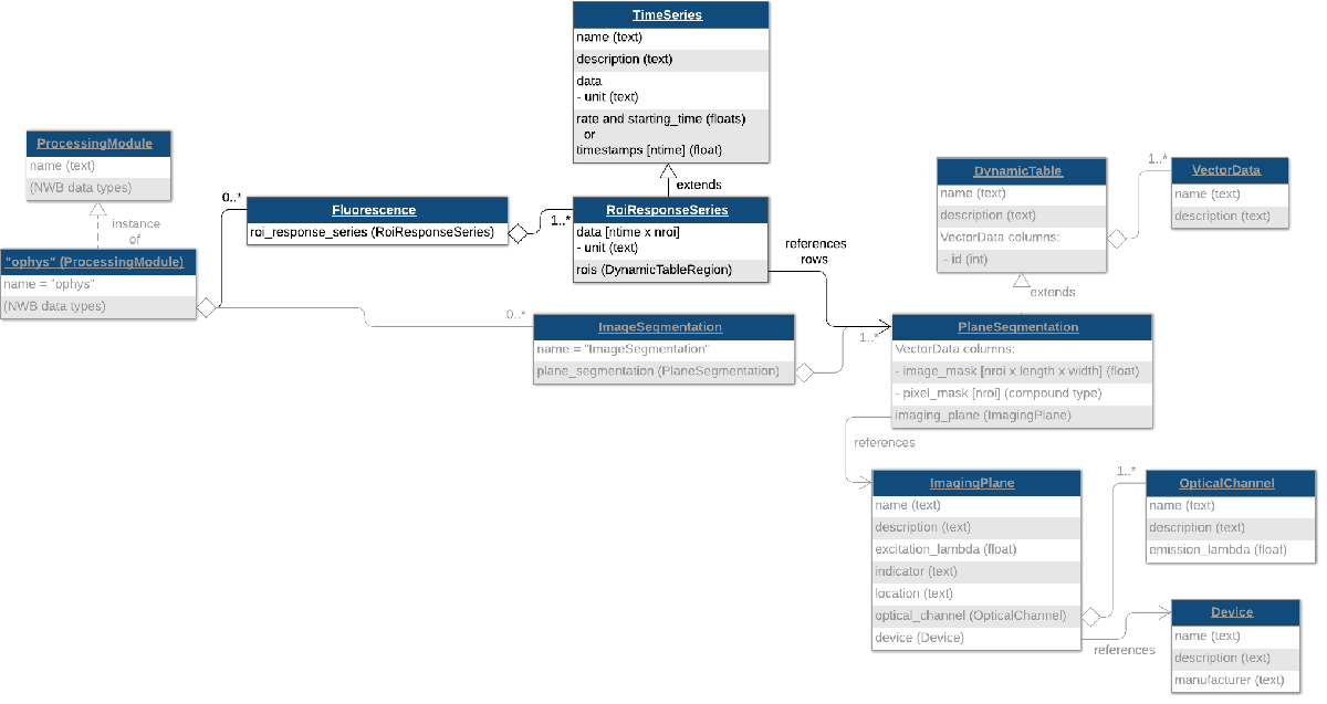
To create a RoiResponseSeries object, we will need to reference a set of rows from the PlaneSegmentation table to indicate which ROIs correspond to which rows of your recorded data matrix. This is done using a DynamicTableRegion, which is a type of link that allows you to reference specific rows of a DynamicTable, such as a PlaneSegmentation table by row indices.
First, we create a DynamicTableRegion that references the ROIs of the PlaneSegmentation table.
roi_table_region = types.hdmf_common.DynamicTableRegion( ...
    'table', types.untyped.ObjectView(plane_segmentation), ...
    'description', 'all_rois', ...
    'data', (0:n_rois-1)');
Then we create a RoiResponseSeries object to store fluorescence data for those ROIs.
data = generateCalciumResponses(n_rois, 100); % [nRoi, nT]
roi_response_series = types.core.RoiResponseSeries( ...
    'rois', roi_table_region, ...
    'data', data, ...
    'data_unit', 'lumens', ...
    'starting_time_rate', 3.0, ...
    'starting_time', 0.0);
To help data analysis and visualization tools know that this RoiResponseSeries object represents fluorescence data, we will store the RoiResponseSeries object inside of a Fluorescence object. Then we add the Fluorescence object into the same ProcessingModule named "ophys" that we created earlier.
fluorescence = types.core.Fluorescence();
fluorescence.roiresponseseries.set('RoiResponseSeries', roi_response_series);

ophys_module.nwbdatainterface.set('Fluorescence', fluorescence);
Tip: If you want to store dF/F data instead of fluorescence data, then store the RoiResponseSeries object in a DfOverF object, which works the same way as the Fluorescence class.
Writing the NWB file
nwb_file_name = 'ophys_tutorial.nwb';
if isfile(nwb_file_name); delete(nwb_file_name); end
nwbExport(nwb, nwb_file_name);
Reading the NWB file
read_nwb = nwbRead(nwb_file_name, 'ignorecache');
Data arrays are read passively from the file. Calling TimeSeries.data does not read the data values, but presents an HDF5 object that can be indexed to read data.
read_nwb.processing.get('ophys').nwbdatainterface.get('Fluorescence')...
    .roiresponseseries.get('RoiResponseSeries').data
ans =
  DataStub with properties:

    filename: 'ophys_tutorial.nwb'
        path: '/processing/ophys/Fluorescence/RoiResponseSeries/data'
        dims: [20 100]
       ndims: 2
    dataType: 'double'
This allows you to conveniently work with datasets that are too large to fit in RAM all at once. Access the data in the matrix using the load method.
load with no input arguments reads the entire dataset:
signals = read_nwb.processing.get('ophys').nwbdatainterface.get('Fluorescence'). ...
roiresponseseries.get('RoiResponseSeries').data.load();
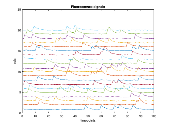
% Plot signals for all RoIs
plot(signals' + (1:size(signals, 1)))
xlabel('timepoints'); ylabel('rois')
title('Fluorescence signals')
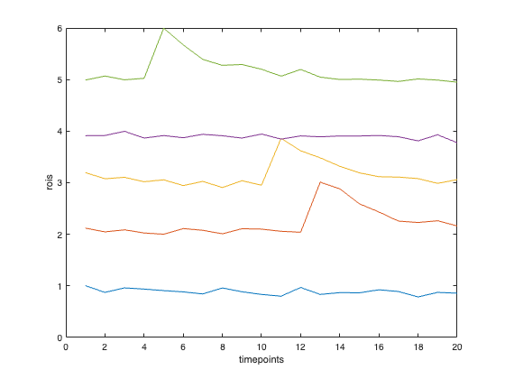
If all you need is a section of the data, you can read only that section by indexing the DataStub object like a normal array in MATLAB. This will just read the selected region from disk into RAM. This technique is particularly useful if you are dealing with a large dataset that is too big to fit entirely into your available RAM.
signal_subset = read_nwb.processing.get('ophys'). ...
    nwbdatainterface.get('Fluorescence'). ...
    roiresponseseries.get('RoiResponseSeries'). ...
    data(1:5, 1:20);

% Plot signals for a subset of RoIs and timepoints
plot(signal_subset' + (1:size(signal_subset, 1)))
xlabel('timepoints'); ylabel('rois')
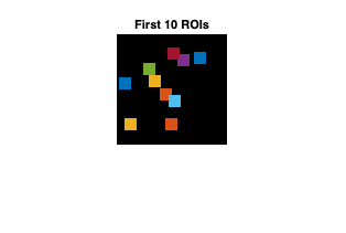
Finally, read back the image/pixel masks and display the first 10 RoIs in a figure:
plane_segmentation = read_nwb.processing.get('ophys'). ...
    nwbdatainterface.get('ImageSegmentation'). ...
    planesegmentation.get('PlaneSegmentation');

num_rois = plane_segmentation.id.data.dims(1);

% Replace this with the correct image size if needed
% Example: imaging_shape = [512, 512];
label_image = zeros(imaging_shape);

for i = 1:10
    if ~isempty(plane_segmentation.image_mask)
        % image_mask is assumed to be height x width x nRois
        image_mask_data = plane_segmentation.image_mask.data;
        roi_mask = image_mask_data(:,:,i) > 0;
        label_image(roi_mask) = i;

    elseif ~isempty(plane_segmentation.pixel_mask)
        row = plane_segmentation.getRow(i, 'columns', {'pixel_mask'});
        pixel_mask = row.pixel_mask{1};

        % pixel_mask is assumed to have fields x, y, and weight
        ind = sub2ind(imaging_shape, pixel_mask.y, pixel_mask.x);

        % Mark ROI pixels with the ROI index
        label_image(ind) = i;
    end
end

rgb_image = convertLabelImage2RGBImage(label_image); % Local helper function

imshow(rgb_image)
title(sprintf('First %d ROIs', 10))
Learn more!
See the API documentation to learn what data types are available.
Other MatNWB tutorials
Python tutorials
See our tutorials for more details about your data type:
Check out other tutorials that teach advanced NWB topics:
Helper functions
function X = generateCenterCoords(varargin)
    % Use reproducible random number generation for consistent
    % tutorial output and export.
    rndGeneratorState = rng(2, 'twister');
    rngCleanup = onCleanup(@() rng(rndGeneratorState));
    X = randi(varargin{:});
end

function data = generateCalciumResponses(nRois, nTime)
    arguments
        nRois (1,1) double {mustBeInteger, mustBePositive}
        nTime (1,1) double {mustBeInteger, mustBePositive}
    end

    % Use reproducible random number generation for consistent
    % tutorial output and export.
    rndGeneratorState = rng(2, 'twister');
    rngCleanup = onCleanup(@() rng(rndGeneratorState));

    data = zeros(nRois, nTime);

    eventProbability = 0.05;
    decayTimeConstant = 3;                 % samples
    kernelLength = 16;                     % samples

    kernel = exp(-(0:kernelLength-1) / decayTimeConstant);

    for i = 1:nRois
        spikeTrain = rand(1, nTime) < eventProbability;
        response = conv(double(spikeTrain), kernel, "same");
        noise = 0.05 * randn(1, nTime);
        baseline = 0.1 * randn;

        data(i, :) = baseline + response + noise;
    end
end

function rgbImage = convertLabelImage2RGBImage(labelImage)
    numLabels = numel(unique(labelImage(labelImage>0)));

    % Create one distinct color per label
    cmap = lines(numLabels);

    % Convert label image to RGB
    map = [0 0 0; cmap]; % black for background plus label colors
    rgbImage = reshape(map(labelImage(:)+1, :), [size(labelImage), 3]);
end